
Reverse-Engineering 20 Smart Beta ETFs — What the Data Reveals
A Python-powered factor analysis showing which funds truly deliver on their promises… and which quietly drift away from their label.

ARTICLE UPDATE: Hello readers! I updated this article with code that calculates the Low Volatility Factor returns ourselves, other than pulling the data directly. Happy reading and have a good week ahead!
Today we are going to look at factor investing, which is one of the most important ideas in modern investing. Factor investing breaks down what really drives stock returns — beyond just buying the whole market. Instead of guessing, factor investing focuses on systematic traits like value, momentum, quality, or size that research shows offer insights into why some stocks consistently outperform and help explain reveal the hidden drivers of equity performance.
In recent years, Smart Beta ETFs are getting more and more popular. They try to give you exposure to one or more of the above-mentioned time-tested factors using a rules-based strategy at low cost. But do they actually deliver what they claim?
👉 GET THE PYTHON NOTEBOOK for the full analysis in this post here.
In this article, we’ll put that to the test.
Using Python and a multi-factor regression model, we’ll reverse-engineer a wide set of popular Smart Beta ETFs, in fact 20 of them, to uncover what they’re really tracking under the hood.
Before we dive in, let’s briefly talk about factor investing and its history.
What Is Factor Investing, and Where Did It Come From?
Back in the 1990s, two finance professors, Eugene Fama and Kenneth French, noticed that some types of stocks kept doing better than others, but the standard model used back then to explain stock returns could not fully explain why.
At the time, most investors relied on something called the Capital Asset Pricing Model (CAPM), which basically said:
“The more market risk you take (as measured by how much your stock moves with the market), the more return you should get.”
But Fama and French saw that small companies and “cheap” stocks (based on their book value) were consistently beating the market (something that CAPM didn’t predict).
So in 1993, they proposed a new, improved model with 3 key ingredients:
Market risk (same as CAPM)
Size (small companies tend to do better)
Value (cheap stocks with low P/B ratios tend to outperform expensive ones)
Later in 2015, they improved it further by adding two more:
Profitability (more profitable companies perform better)
Investment behavior (companies that try to grow conservatively tend to outperform those that invest aggressively to grow)
These became known as the Fama-French 5 Factors.
Over the years, other researchers and data-driven investors added even more ideas, like Momentum (stocks that have gone up tend to keep going up) and Low Volatility (less risky stocks can sometimes give better returns than risky ones!). In fact, hundreds of factors have now emerged but we will just focus on the more widely established ones in this article.
Feel free to read more about its history here.
Once you have collected all the factors in the universe as shown below, all you need to do is to snap your fingers and your portfolio will double (I’m kidding, sorry for the lame joke, just a hardcore Marvel fan here).

Smart Beta ETFs
Today, these ideas are at the heart of Factor Investing and you no longer need to be a quant hedge fund to try it, thanks to Factor-Based funds and more recently, Smart Beta ETFs.
Instead of blindly following market cap like traditional index funds, Smart Beta ETFs are marketed to tilt toward specific styles so investors can try to capture those long-term advantages.
In this article, we’ll dive into what these factors are — and as mentioned earlier, we will use Python to analyze whether Smart Beta ETFs actually deliver on what they promise.
Let’s dive right in. Here’s our set-up:
import zipfile
import os
from io import BytesIO

# for performing regression
import statsmodels.api as sm

# for data processing
import pandas as pd
import numpy as np

# for plotting
import matplotlib.pyplot as plt
import seaborn as sns
import plotly.express as px

# for coloring heatmaps later
from matplotlib.colors import LinearSegmentedColormap
from matplotlib.colors import TwoSlopeNorm
from matplotlib.colors import ListedColormap

# for fetching data
import requests
from urllib.request import urlopen
import json

# for fetching json data from FMP API
def get_jsonparsed_data(url):
    resp = urlopen(url); data = resp.read().decode("utf‑8")
    return json.loads(data)
Get Factors Data from Kenneth French’s Data Library
We will now write functions to download and process the factors’ monthly return data directly from Kenneth French’s data library.
If you scroll down this page, you will see the data are in zipped folders of csv files. The code below links directly to the file that we want and handles the unzipping.
def get_factors_dartmouth(filename):
    factors_url = f"https://mba.tuck.dartmouth.edu/pages/faculty/ken.french/ftp/{filename}"
    extract_to = "ff_factors" # folder to extract factor data to, as it will be a zip file
    os.makedirs(extract_to, exist_ok=True) # create the fodler

    resp = requests.get(factors_url); resp.raise_for_status()
    with zipfile.ZipFile(BytesIO(resp.content)) as z: # unzip the file
        z.extractall(extract_to)

    # read CSV file
    csv_filename = filename.replace("_CSV.zip", ".csv") # convert zip filename to csv filename
    file_path = os.path.join(extract_to, csv_filename)
    with open(file_path, "r") as f:
        lines = f.readlines()
    return lines
After reading the lines from the csv file, we write another function to process these lines.
Before we look at the code, let’s understand how our files look like. A screenshot of one of our csv files is shown below. There is a header description which we will eventually need to remove using skiprows in the code below.
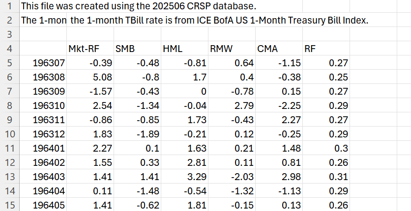
Halfway through the csv file, after the monthly return data, we start to see the annual returns data. We do not need this, so we will stop reading our file after we see the “Annual Factors” line. This is handled in the code below too, where we break the loop after getting to this line (we pass the “Annual Factors” in skip_text when using this function later).
We also parse the dates and make sure it is in the monthly format.
def process_factors_dartmouth(lines, skiprows, skip_text):
    # stop before skip_text line is reached
    cleaned = []
    for line in lines:
        if line.strip().startswith(skip_text): # e.g. Annual Factors
            break
        cleaned.append(line)

    monthly_csv = BytesIO("".join(cleaned).encode())
    df_factors = pd.read_csv(monthly_csv, skiprows=skiprows, index_col=0) # rows are skipped to avoid description in the CSVs
    df_factors = df_factors.iloc[:-1]  # drop footer

    # parse datetime and set it as index
    df_factors.index = pd.to_datetime(df_factors.index, format="%Y%m")
    df_factors.index = df_factors.index.to_period("M") # change to monthly period
    return df_factors
Get Fama French 5 Factors Data from Kenneth French’s Data Library
Let’s obtain the monthly returns of our first 5 factors, this is the well-known Fama-French 5 Factors, it is given inside the Developed_5_Factors_CSV.zip file. A description of the data is given here. There are 4 rows in the header description which we skip.
lines = get_factors_dartmouth("Developed_5_Factors_CSV.zip")
# stop before "Annual Factors" line is reached
# we only want the month factors, so we do not read the section starting from "Annual Factors" onwards
# skiprows so we won't read the description at the start
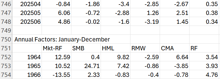
df_5_factors = process_factors_dartmouth(lines, skiprows=4, skip_text = "Annual Factors")
df_5_factors
The RF column above simply stands for the risk-free returns, but what do the rest of the columns mean? They represent percentage returns of each of the factors explained below.
1. Mkt-RF (Market Returns — Risk Free Rate)
The return of the overall stock market minus the risk-free rate (typically 1-month Treasury bill).
A positive Mkt-RF return means the market outperform the Treasury bill returns that month.
2. SMB (Small Minus Big) — Size Factor
SMB captures the size premium: the tendency for small‑cap stocks to outperform large‑cap stocks.
Stocks are first divided into Small and Big based on their market capitalisation.
Within each size group, stocks are further split by other characteristics (value, profitability, investment) to control for those effects.
SMB is the average return of small‑stock portfolios minus big‑stock portfolios across these sorts (this cancels out the influence of other factors so SMB reflects a pure size premium).
A positive SMB means small‑caps outperformed large‑caps that month.
3. HML (High Minus Low) — Value Factor
HML captures the value premium: the tendency for high book‑to‑market (“value”) stocks to outperform low book‑to‑market (“growth”) stocks.
Stocks are first divided into High and Low based on their book‑to‑market ratios.
Within each value group, stocks are further split into size (Small and Big) to control for the size effect.
HML is the average return of high book‑to‑market portfolios minus low book‑to‑market portfolios across these size groups (across size so this cancel out the size effect so HML reflects a pure value premium).
HML = 1/2 (Small Value + Big Value) — 1/2 (Small Growth + Big Growth)
A positive HML return means value stocks beat growth stocks that month.
4. RMW (Robust Minus Weak) — Profitability/Quality Factor
RMW captures the profitability premium: more profitable firms tend to generate higher returns. This is often included in quality factors also so we will use this as proxy for the quality factor.
Stocks are first divided into Robust and Weak based on their operating profitability.
Within each profitability group, stocks are further split into size (Small and Big) to control for the size effect.
RMW is the average return of robust‑profitability portfolios minus weak‑profitability portfolios across these size groups (this cancels out the size effect so RMW reflects a pure profitability premium).
RMW = 1/2 (Small Robust + Big Robust) − 1/2 (Small Weak + Big Weak)
A positive RMW means profitable companies outperformed unprofitable ones that month.
5. CMA (Conservative Minus Aggressive) — Investment Factor
CMA captures the investment premium: the tendency for firms with low asset growth (conservative investment) to outperform firms with high asset growth (aggressive investment).
Stocks are first divided into Conservative and Aggressive based on their prior asset growth.
Within each investment group, stocks are further split into size (Small and Big) to control for the size effect.
CMA is the average return of conservative‑investment portfolios minus aggressive‑investment portfolios across these size groups (this cancels out the size effect so CMA reflects a pure investment premium).
CMA = 1/2 (Small Conservative + Big Conservative) − 1/2 (Small Aggressive + Big Aggressive)
A positive CMA means low-investment firms outperformed those with high investment rates.
Get Momentum Factor Data from Kenneth French’s Data Library
Let’s do the same thing for the momentum factor monthly returns, inside the F-F_Momentum_Factor_CSV.zip file. A description of the data is given here.
lines = get_factors_dartmouth("F-F_Momentum_Factor_CSV.zip")
# stop before "Annual Factors" line is reached
# we only want the month factors, so we do not read the section starting from "Annual Factors" onwards
# skiprows so we won't read the description at the start
df_factors_mom = process_factors_dartmouth(lines, skiprows=13, skip_text = "Annual Factors")
df_factors_mom = df_factors_mom.rename(columns = {'Mom':'MOM'})
df_factors_mom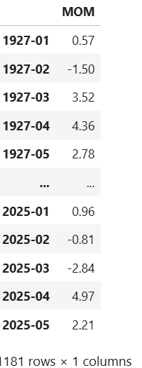
There you go, the momentum factor.
6. MOM (Momentum) — Momentum Factor
MOM captures the momentum premium: the tendency for stocks with strong recent performance to continue outperforming, and for stocks with weak recent performance to continue underperforming.
Stocks are first divided into Winners and Losers based on their prior 12‑month returns (excluding the most recent month).
Within each momentum group, stocks are further split into size (Small and Big) to control for the size effect.
MOM is the average return of winner portfolios minus loser portfolios across these size groups (this cancels out the size effect so MOM reflects a pure momentum premium).
MOM = 1/2 (Small Winners + Big Winners) − 1/2 (Small Losers + Big Losers)
A positive MOM means recent winners outperformed recent losers that month.
Get Low Variance Portfolio Data from Kenneth French’s Data Library
The low volatility factor returns are not available directly in Kenneth French’s data library. But we can calculate it ourselves using one of the datasets that contains low variance portfolio data, which is given in the 25_Portfolios_ME_VAR_5x5_CSV.zip file. A description of the data is given here.
lines = get_factors_dartmouth("25_Portfolios_ME_VAR_5x5_CSV.zip")
# stop before "Average Equal Weighted Returns -- Monthly" line is reached
# we only want the Average Value Weighted Returns -- Monthly, so we do not read the section starting from "Annual Factors" onwards
# skiprows so we won't read the description at the start
df_portfolio_size_var = process_factors_dartmouth(lines, skiprows=19, skip_text = "Average Equal Weighted Returns -- Monthly")
df_portfolio_size_var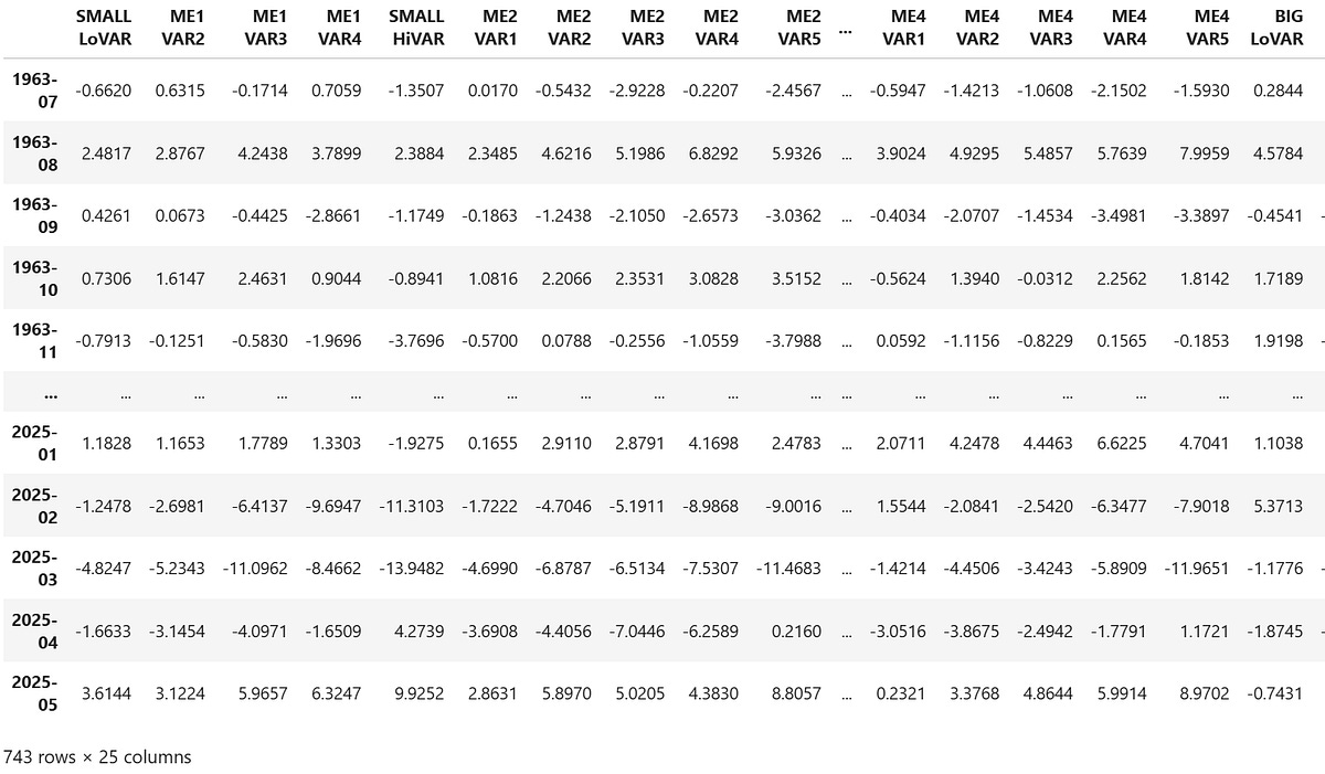
Calculate Low Volaility Factor Data Ourselves
Now that we have the dataset of portfolios formed on size and variance, we calculate the low volatility factor returns ourselves.
Remember how the other factors were calculated? For example the value factor was calculated like this: HML = 1/2 (Small Value + Big Value) — 1/2 (Small Growth + Big Growth).
We would calculate our low volatility factor in a similar way.
7. VOL (Volatility) — Low-Volatility Factor
VOL captures the low‑volatility premium: the tendency for low‑volatility stocks to outperform high‑volatility stocks.
Stocks are first divided into Low Volatility and High Volatility based on their past realised volatility (or variance).
Within each volatility group, stocks are further split into size (Small and Big) to control for the size effect.
VOL is the average return of low‑volatility portfolios minus high‑volatility portfolios across these size groups (this cancels out the size effect so VOL reflects a pure low‑volatility premium).
VOL = 1/2 (Small Low Vol + Big Low Vol) − 1/2 (Small High Vol + Big High Vol)
A positive VOL means low‑volatility stocks outperformed high‑volatility stocks that month.
Our data above has already split portfolios by size and variance. Let’s do the calculation in code. Note that low volatility and high volatility are similar to low variance and high variance portfolios respectively.
df_portfolio_size_var['VOL'] = (
    (df_portfolio_size_var['SMALL LoVAR'] + df_portfolio_size_var['BIG LoVAR']) / 2
    - (df_portfolio_size_var['SMALL HiVAR'] + df_portfolio_size_var['BIG HiVAR']) / 2
)
df_portfolio_size_var[['VOL']]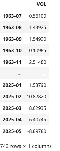
There we go!
Concatenate All Factors
Let’s concatenate all 7 factors we have obtained into the df_factors DataFrame.
df_factors = df_5_factors.merge(df_factors_mom, left_index=True, right_index=True).merge(df_portfolio_size_var[['VOL']], left_index=True, right_index=True)
earliest_date = df_factors.index[0].strftime('%Y-%m-%d') # capture earliest date that we will use to pull the ETF data later
df_factors = df_factors.apply(pd.to_numeric)
df_factors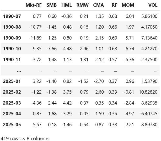
We now have a good solid 30+ years of factor returns data, more than enough to run regressions against the Smart Betas ETFs. These ETFs themselves haven’t been around for the entire period. Note that the most recent factor data available is only till May 2025, meaning our regression can only be performed till then. That is quite recent and not a big problem.
Correlation Matrix of Factors
Let’s look at the correlation among each of the factors first.
# for coloring heatmap (more positive = darker green and more negative = darker red)
rdgn = sns.diverging_palette(h_neg=10, h_pos=130, s=99, l=55, sep=3, as_cmap=True)
divnorm = TwoSlopeNorm(vmin=-1, vcenter=0, vmax=1)

plt.figure(figsize=(6, 5))
sns.heatmap(
    df_factors.corr(), # get the correlation matrix of factors
    annot=True,
    fmt=".2f",
    cmap=rdgn,
    linewidths=0.5,
    cbar_kws={"label": "Correlation"}
)

plt.title("Heatmap of Correlation Among Factors")
plt.tight_layout()
plt.show()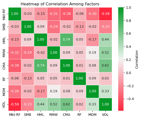
This heatmap shows the correlation among all the factors.
Most of the factors are not THAT highly correlated with each other. This is good because this helps to avoid multicollinearity to some extent when running a multi-factor regression, an issue where overlapping variables distort the true effect of each factor.
If you have seen a heatmap of the correlation between individual stocks, you often see way higher values than these.
Some Values Stand Out Though
BUT the correlations are not 0 either, we note that there are still a few stronger correlation values that stand out above. Let’s try to explain some of them to see if they make sense:
Market risk premium vs quality/profitability (RMW) (-0.32): High-quality, profitable companies can be more defensive and tend to underperform in strong bull markets (especially those led by more speculative growth stocks) and outperform in bear markets. Hence the negative correlation.
Market risk premium vs investment (CMA) (-0.38): Conservative asset growth is often seen in mature businesses which can also underperform when markets are roaring, compared to younger busineses investing aggressively, and outperform in bear markets.
Market risk premium vs momentum (MOM) (-0.30): This is likely due to momentum being sensitive to trend reversals. In sharp crashes, momentum often fails badly, producing negative correlation in those periods and vice versa for sharp rebounds.
Market risk premium vs low volatility (VOL) (-0.58): In strong bull markets, the low-vol factor usually underperforms as investors prefer higher-risk stocks, pushing the market risk premium higher. On the other hand, the low-volatility factor tends to perform better in down markets when investors flock to safer, less-volatile stocks. This naturally creates an inverse relationship.
Size (SMB) vs profitability (RMW) (-0.29): Remember size means the returns of smaller firms minus larger firms. Smaller firms, on average, are less profitable and more speculative. Quality/profitability factor tends towards larger, cash-generating companies, so the small MINUS BIG part of the returns makes it negatively correlated to the larger companies.
Size (SMB) vs low volatility (VOL) (-0.23): Smaller companies are more highly volatile, I think we have all observed that before. So they are negatively correlated to LOW volatility factor.
Value (HML) vs investment (CMA) (+0.74): This one is strongly positive. Likely because cheap stocks (high book/market value) are often also asset-heavy mature companies that don’t reinvest aggressively, so value and conservative investment tend to reinforce each other.
Value (HML) and investment (CMA) factors are positively correlated to low volatily (VOL) (+0.44 and +0.62): Cheap firms and firms that invest cautiously tend to be more stable and “unexciting”, and less sensitive to speculative market manias than growth stocks, hence the lower volatility.
Profitability (RMW) vs low volatility (VOL) (+0.52): Profitable firms usually have steady cash flows and better margins. This reduces the uncertainty in their future earnings, so there is lower volatility in their stock prices too.
From here, we should keep in mind that:
In targetting certain factors, other factors may sometimes also be inevitably “dragged in” as we see some correlation between a few of them.
Obtain ETF Prices and Computing Returns
Historical ETF prices data can be obtained from the Financial Modeling Prep API for free. You need to sign up for an account here to get an API key (250 requests per day for the free tier). After signing up, your API key will be shown on the dashboard (access it with the button at the top right).
Enter your API key in the next cell to store it in the environment variable “FMP_API_KEY”. We will use it for our requests later.
# uncomment and enter API Key below
# os.environ['FMP_API_KEY'] = "YOUR_API_KEY"
api_key = os.environ['FMP_API_KEY']
Let’s first fetch the prices, using the "VBR" ETF (Vanguard Small Cap Value ETF) as an example.
# fetch returns for symbol (from "earliest date" of factor data)
symbol = "VBR"
url = f"https://financialmodelingprep.com/stable/historical-price-eod/full?symbol={symbol}&from={earliest_date}&apikey={api_key}"
raw = get_jsonparsed_data(url)
df = pd.DataFrame(raw).iloc[::-1]  # reverse chronological
df["date"] = pd.to_datetime(df["date"])
df.set_index("date", inplace=True)
df
We get the daily returns below, and notice that this ETF only began trading in 2004.
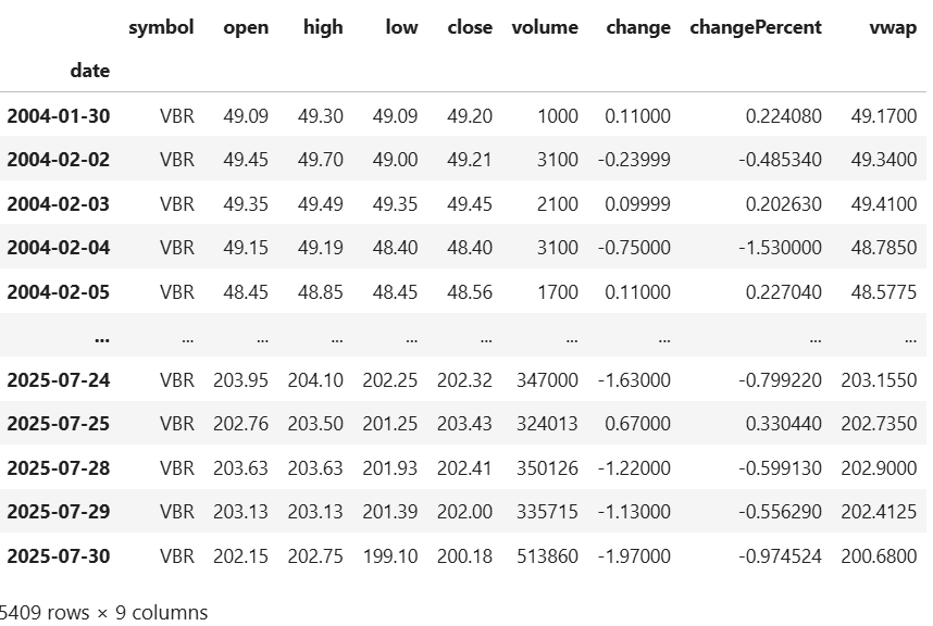
We need to get the percentage returns data and resample them to monthly returns, like our factor data.
# compute monthly returns
monthly = ((1 + df["close"].pct_change()).resample("ME").prod() - 1).dropna()
monthly = monthly.to_frame("return")
monthly.index = monthly.index.to_period("M") # change to monthly period
monthly
We then calculate the excess returns over the risk free rate and store it in the excess column, this is what we will regress against the factor returns. We also merge this data with the df_factors data.
# merge price data with factor data
df_reg = monthly.join(df_factors, how="inner")
df_reg["excess"] = df_reg["return"] * 100 - df_reg["RF"] # excess returns above risk free rate
df_reg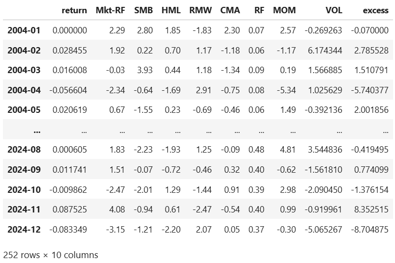
Let’s first copy the above code for our data pulling and processing into the function analyze_etf below.
def analyze_etf(symbol, name, df_factors):
    # fetch returns for symbol (from "earliest date" of factor data)
    url = f"https://financialmodelingprep.com/stable/historical-price-eod/full?symbol={symbol}&from={earliest_date}&apikey={api_key}"
    raw = get_jsonparsed_data(url)
    df = pd.DataFrame(raw).iloc[::-1]  # reverse chronological
    df["date"] = pd.to_datetime(df["date"])
    df.set_index("date", inplace=True)

    # compute monthly returns
    monthly = ((1 + df["close"].pct_change()).resample("ME").prod() - 1).dropna()
    monthly = monthly.to_frame("return")
    monthly.index = monthly.index.to_period("M") # change to monthly period

    # merge price data with factor data
    df_reg = monthly.join(df_factors, how="inner")
    df_reg["excess"] = df_reg["return"] * 100 - df_reg["RF"] # excess returns above risk free rate    # perform regression
Perform Multi-Factor Regressions Against Smart Beta ETFs
This is the regression function we are working with. Hopefully you can see how each variable corresponds to the columns in our final DataFrame above.
Excess Return of ETF = α + β₁·(Mkt-RF) + β₂·SMB + β₃·HML + β₄·RMW + β₅·CMA + β₆·MOM + β₇·VOL + error
where:
ETF Excess Return = the ETF’s return minus the risk-free rate
Mkt-RF = the equity market premium (Market — Risk-Free)
SMB = Small Minus Big (size factor)
HML = High Minus Low (value factor)
RMW = Robust Minus Weak (profitability factor) (often included in quality factor also)
CMA = Conservative Minus Aggressive (investment factor)
MOM = Momentum factor
VOL = Low Volatility factor
α = intercept (alpha) (returns that are unexplained by factors alone)
β₁ to β₇ = beta coefficients of each facor, i.e. the ETF’s exposure (or “loading”) to each factor
error = random residual not explained by the model
The code below shows the continuation of our analyze_etf function. We use the statsmodels library to run an ordinary least squares regression. The we extract the beta coefficients, betas, and their t-values.
t-values
I won’t dive deeply into t-values here, but just know that t-values help us understand how confident we can be about each beta. A high absolute t-value (typically above 2) suggests that the beta coefficient of a factor is statistically significant, meaning the corresponding factor likely has a real and meaningful impact on the ETF’s returns, rather than just being due to noise or chance.
Betas
For now, our focus is on the betas — these are the estimated exposures of the ETF to each factor. A high positive beta means the ETF behaves similarly to that factor (e.g. it might be tilted toward small caps or value stocks), while a negative beta means it tends to move in the opposite direction of that factor.
    # perform regression
    X = sm.add_constant(df_reg[["Mkt-RF","SMB","HML","MOM","RMW", "CMA", "VOL"]])
    y = df_reg["excess"]

    model = sm.OLS(y, X).fit()

    # extract betas
    betas = model.params.drop("const")

    # store betas in dataframe for plotting
    df = betas.rename_axis("factor").reset_index(name="beta")

    # capture t-stats
    tstats = model.tvalues.drop("const").reindex(df["factor"]).values
Plot the Beta Coefficients
In the remaining part of the analyze_etf function, we plot the betas on a bar chart and we also label these values, and their respective t-values inside the chart. Because betas with |t| < 2 are statistically insignificant, we make their bars more translucent and faded. We will see how these translate into our charts later!
    # plotly bar chart
    fig = px.bar(
        df_plot,
        x="factor",
        y="beta",
        text='beta',
        orientation="v",
        color="factor",
        range_color=[-1, 1],
        title=f"{name} ({symbol}) Factors"
    )

    fig.update_traces(
        texttemplate='%{text:.2f}',   # format the beta label to two decimals
        textposition='outside'        # place beta above each bar
    )

    fig.update_layout(
        xaxis_title="",
        yaxis_title="Beta",
        template="plotly_white",
        width=600,
        height=600,
        showlegend=False,
        yaxis=dict(range=[-0.8, 1.25]) # fix scale so its easier to compare across plots
    )

    # append t-values underneath each factor label
    fig.update_xaxes(
        tickvals=df_plot["factor"],
        ticktext=[f"{f}\n(t={t:.2f})" for f, t in zip(df_plot["factor"], tstats)] # label the x axis with the t values also
    )

    # make bars with |t| < 2 more translucent
    for idx, t in enumerate(tstats):
        fig.data[idx].update(marker_opacity=0.2 if abs(t) < 2 else 1.0)

    fig.show()

    return betas, tstats
List ETFs of Interest
Let’s look at all the ETFs that I have decided to look at, feel free to add more if you want. I have included a short description of each of the funds to see which specific factors they are targetting.
Ok, I admit, we are not just looking at Smart-Beta funds per se, but also ETFs like SPY to see which factors they tilt towards.
I have arranged the funds by the factors they are targetting, and provided at least 2 funds for each factor so we can compare between funds that are targetting the same factors. Towards the end of the list I have also included some multi-factor funds.
# all the etfs
etf_data = [
    # Small Cap
    {"Symbol": "VBR",  "Name": "Vanguard Small Cap Value ETF",
     "Description": "Tracks the CRSP US Small Cap Value Index",
    },
    {"Symbol": "IJR", "Name": "iShares Core S&P Small-Cap ETF",
     "Description": "Tracks the S&P SmallCap 600 Index",
    },

    # Large Cap and Core Market
    {"Symbol": "USMC", "Name": "Principal U.S. Mega-Cap ETF",
     "Description": "Tracks an index of the largest U.S. companies",
    },
    {"Symbol": "SPY",  "Name": "SPDR S&P 500 ETF",
     "Description": "Tracks the S&P 500 Index (market-cap weighted broad large-cap fund)",
    },
    {"Symbol": "RSP",  "Name": "Invesco S&P 500 Equal Weight ETF",
     "Description": "Allocates equal weights to S&P 500 constituents, removing market-cap tilt",
    },

    # Value
    {"Symbol": "RPV",  "Name": "Invesco S&P 500 Pure Value ETF",
     "Description": "Invests in the highest book-to-market decile of S&P 500 stocks",
    },
    {"Symbol": "IUSV", "Name": "iShares Core S&P U.S. Value ETF",
     "Description": "Tracks the S&P USA Value Index (value-tilted large-cap portfolio)",
    },
    {"Symbol": "VTV",  "Name": "Vanguard Value ETF",
     "Description": "Tracks the CRSP US Large Cap Value Index (value-tilted large-cap fund)",
    },
    {"Symbol": "VLUE", "Name": "iShares MSCI USA Value Factor ETF",
     "Description": "Weights large- and mid-cap equities using earnings, revenue, book value and cash-flow metrics to emphasize undervalued stocks",
    },
    {"Symbol": "HDV",  "Name": "iShares Core High Dividend ETF",
     "Description": "Tracks the Morningstar Dividend Yield Focus Index, targeting high-yielding large-cap companies with value characteristics",
    },

    # Quality
    {"Symbol": "QUAL", "Name": "iShares MSCI USA Quality Factor ETF",
     "Description": "Selects large- and mid-cap stocks based on stable earnings growth and low debt-to-equity",
    },
    {"Symbol": "QGRO", "Name":   "American Century U.S. Quality Growth ETF",
     "Description": "Tracks the American Century U.S. Quality Growth Index, selecting large- and mid-cap U.S. companies with strong quality, growth, and valuation fundamentals",
    },
    {"Symbol": "JQUA", "Name": "JPMorgan U.S. Quality Factor ETF",
     "Description": "Selects U.S. stocks with high profitability, stable earnings growth, and low financial leverage to capture the quality premium"
    },

    # Momentum
    {"Symbol": "MTUM", "Name": "iShares MSCI USA Momentum Factor ETF",
     "Description": "Holds large-cap U.S. stocks that exhibit positive price momentum",
    },
    {"Symbol": "VFMO", "Name": "Vanguard U.S. Momentum Factor ETF",
     "Description": "Tilts toward U.S. stocks exhibiting strong recent price momentum, selecting winners via a rules-based momentum screen"
    },

    # Low Volatility
    {"Symbol": "USMV", "Name": "iShares Edge MSCI Min Vol USA ETF",
     "Description": "Tracks an index of U.S. stocks with the lowest realized volatility, aiming to smooth returns and reduce downside risk"
    },
    {"Symbol": "SPLV", "Name": "Invesco S&P 500 Low Volatility ETF",
     "Description": "Selects the 100 least volatile stocks from the S&P 500",
    },

    # Multi-Factor ETFs
    {"Symbol": "LRGF", "Name": "iShares US Equity Factor ETF",
     "Description": "Selects large- and mid-cap U.S. stocks to maximise exposure to momentum, quality, value, low volatility and size",
    },
    {"Symbol": "GSLC", "Name": "Goldman Sachs ActiveBeta US Large Cap Equity ETF",
     "Description": "Targets value, momentum, quality and low volatility in large-cap U.S. stocks",
    },
    {"Symbol": "VFMF", "Name": "Vanguard U.S. Multifactor ETF",
     "Description": "Tilts toward value, momentum, quality and low volatility across U.S. equities",
    },
]


df_etf = pd.DataFrame(etf_data)
Perform Regression on Each ETF
Let’s loop through each ETF and do the regression!
betas_list = []

# loop through all ETFs and store their betas
for idx, row in df_etf.iterrows():
    print(f"{row['Symbol']}: {row['Name']} - {row['Description']}")
    # Run regression & get betas Series
    beta = analyze_etf(row['Symbol'], row['Name'], df_factors)
    # Name the Series by symbol for indexing
    beta.name = row['Name']
    betas_list.append(beta)

# Combine into a single DataFrame
all_betas = pd.DataFrame(betas_list)
all_betas.index.name = 'Name'
Here are our results, we will analyze these ETFs in groups, according to what factors they target. Once again, recall that some bars below are more translucent and faded as they have |t| < 2 and are statistically insignificant. Also notice that Mkt‑RF has the highest beta for all of them, we will ignore that for now and come back to it towards the end of the article.
To keep things concise, I’ll use SMB, HML, RMW, CMA, MOM, and VOL to denote their beta coefficients directly, in this part of the article.
Small Cap ETFs
VBR: Vanguard Small Cap Value ETF
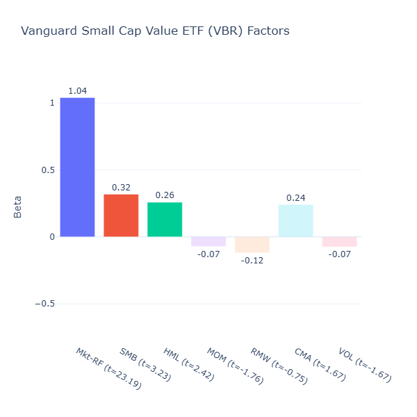
ETF Description: Tracks the CRSP US Small Cap Value Index
As expected, VBR shows both a positive size tilt (SMB = 0.32, t = 3.23) and a clear value tilt (HML = 0.26, t = 2.42). This is what you want from a small‑cap value fund. Note: Recall that a positive beta for the size factor means small-caps are favoured (SMB means small minus big). The rest of the factors are statistically insignificant (|t| < 2).
IJR: iShares Core S&P Small-Cap ETF
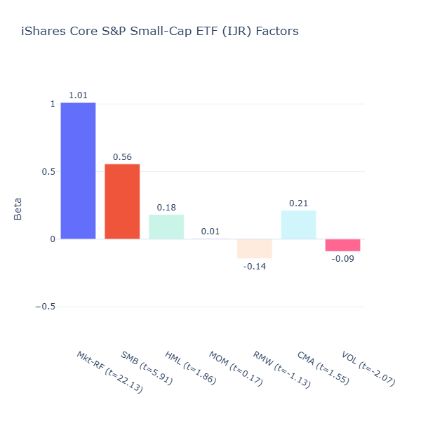
ETF Description: Tracks the S&P SmallCap 600 Index
This fund is a purer small‑cap play (SMB = 0.56, t = 5.91). The rest of the beta coefficients are insignificant except for the small negative low volatility tilt (VOL = -0.09, t = -2.07), which is unsurprising as small caps are more volatile. This ETF makes it more suitable for investors with high-conviction to the size factor and who want a single size factor exposure.
Large Cap and Core Market ETFs
USMC: Principal U.S. Mega-Cap Multi-Factor ETF
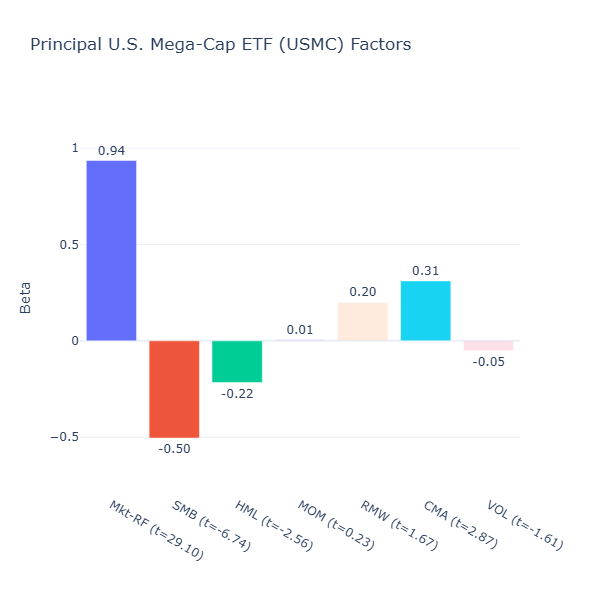
ETF Description: Tracks an index of the largest U.S. companies
USMC’s exposures confirm its mega‑cap orientation with a significant negative size tilt (SMB = –0.50, t = –6.74). In fact it has a growth profile, with a negative value tilt (HML = –0.22, t = –2.56) likely because its biggest holdings include large cap growth companies like MSFT, NVDA and AAPL with higher valuations.
Finally, it has a positive conservative investment tilt (CMA = 0.31, t = 2.87) as large‑caps are more mature and invest less aggressively relative to their large amount of assets.
SPY: SPDR S&P 500 ETF
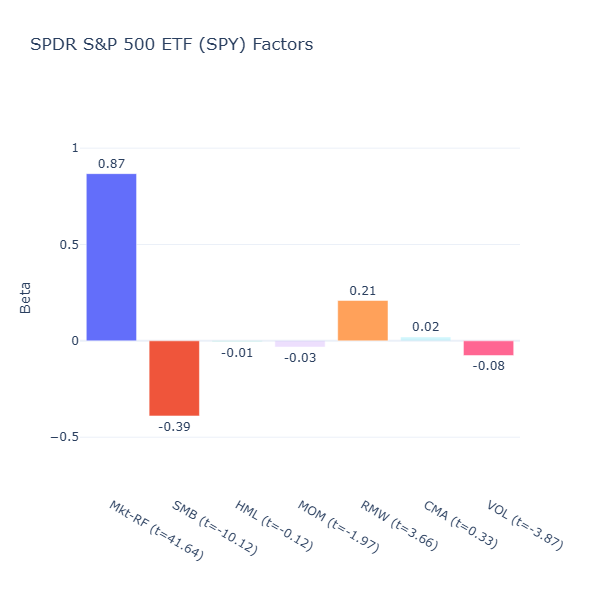
ETF Description: Tracks the S&P 500 Index (market-cap weighted broad large-cap fund)
This is none other than our S&P 500 ETF. We know this ETF to be “tracking the market”, however this ETF does not track the entire broad US market. In fact, we can consider this a large cap ETF as it tracks the leading companies and weighs them by market-cap. Hence it has a negative size tilt (SMB = –0.39, t = –10.12). The S&P 500 is dominated by leaders with consistently high profitability, hence the positive profitability/quality tilt (RMW = 0.21, t = 3.66).
RSP: Invesco S&P 500 Equal Weight ETF
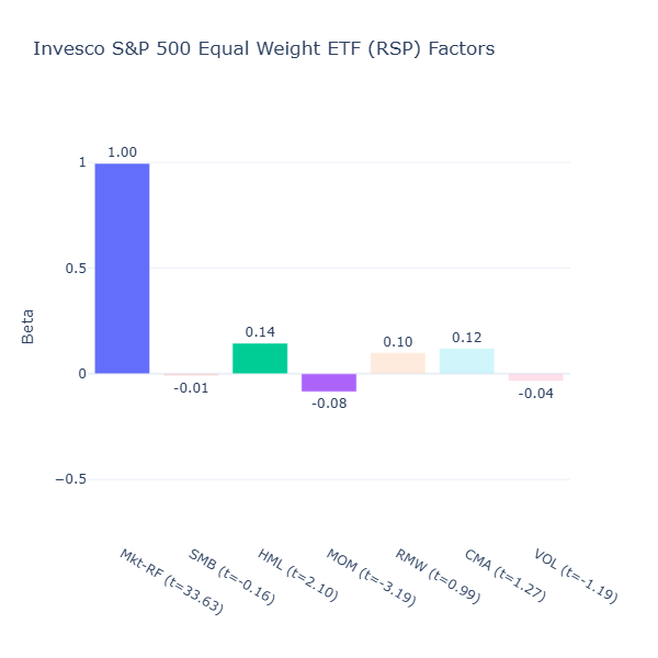
ETF Description: Allocates equal weights to S&P 500 constituents, removing market-cap tilt
This is an interesting one, RSP has the same constituents as SPY but they are equal weighted. This means that larger market cap companies are not given more weight and the relative weight of smaller cap companies are now heavier. Because of this, the negative size tilt that we see in SPY disappears, RSP does not favour large cap stocks.
Moreover, the profitability tilt that we see in SPY disappears as well. Because SPY is market‑cap weighted, those highly profitable giants take up a large share of the index, which is no longer the case here.
It has a slight value tilt (HML = 0.14, t = 2.10) as the equal weighting reduces exposure to high‑valuation mega‑cap tech names compared to SPY.
Comparing Among Size-Oriented ETFs
When comparing all the size‑oriented ETFs, the spectrum runs from pure small‑cap exposure to concentrated mega‑cap bets. On the small‑cap side, IJR is a pure small‑cap vehicle delivering a strong size tilt and little else. VBR blends a solid positive size tilt with a value bias, making it a dual factor ETF.
Moving to the other end, USMC is anchored in mega‑caps with a strong negative size tilt, growth orientation, and a conservative investment profile typical of mature firms. SPY, our well-known S&P 500 tracker, leans large‑cap with some profitability exposure. RSP, its equal‑weight cousin, neutralises that large‑cap bias, offering a more balanced exposure to the market.
Value ETFs
RPV: Invesco S&P 500 Pure Value ETF
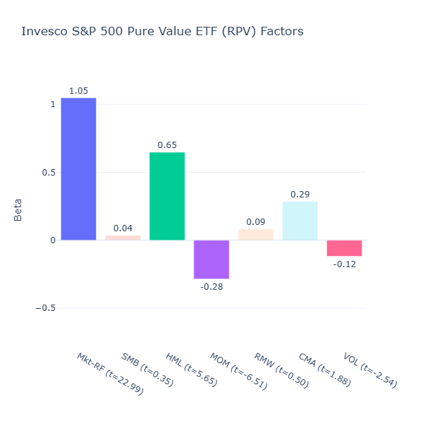
ETF Description: Invests in the highest book-to-market decile of S&P 500 stocks
RPV is what deep value should look like, with a strong value tilt (HML = 0.65, t = 5.65) that comes from focusing on the highest book‑to‑market stocks in the S&P 500. Naturally, these are companies the market has deeply discounted and thus they tend to have lower momentum (MOM = –0.28, t = –6.51) as they’ve underperformed recently.
IUSV: iShares Core S&P U.S. Value ETF
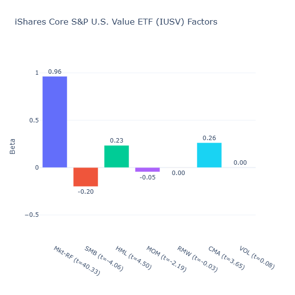
ETF Description: Tracks the S&P USA Value Index (value-tilted large-cap portfolio)
IUSV has a moderate value tilt (HML = 0.23, t = 4.50) and a moderate large‑cap bias (SMB = –0.20, t = –4.06), which is exactly what it is tracking. It also has moderate conservative investment tilt (CMA = 0.26, t = 3.65) as large‑caps value companies are more mature and invest less aggressively relative to their large amount of assets.
VTV: Vanguard Value ETF
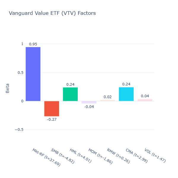
ETF Description: Tracks the CRSP US Large Cap Value Index (value-tilted large-cap fund)
VTV mirrors IUSV in many ways: moderate value tilt (HML = 0.24, t = 4.01), moderate large‑cap bias (SMB = –0.27, t = –4.06) and moderate conservative investment tilt (CMA = 0.24, t = 2.99). So I shan’t elaborate too much here.
VLUE: iShares MSCI USA Value Factor ETF
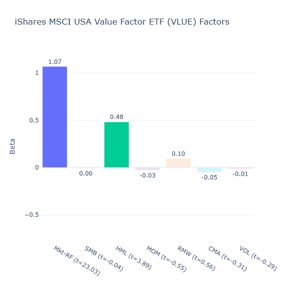
ETF Description: Weights large- and mid-cap equities using earnings, revenue, book value and cash-flow metrics to emphasize undervalued stocks
VLUE offers strong value exposure (HML = 0.48, t = 3.89). I like its clean ticker symbol “VLUE”, and it seems that its value exposure is as pure and clean as its symbol, with little exposure to other factors.
Interestingly, it does not seem to have a negative size tilt despite weighting large and mid cap equities. This is likely because large‑caps today are dominated by high‑growth tech or consumer companies that have expanded rapidly for years. The value-tilt would have favoured a heavier mid‑cap allocation, which offsets the size tilt.
HDV: iShares Core High Dividend ETF
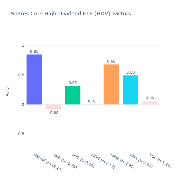
ETF Description: Tracks the Morningstar Dividend Yield Focus Index, targeting high-yielding large-cap companies with value characteristics
High dividend companies often have stable earnings and conservative investment policies (in order to allocate more of their earnings to pay dividends), so there will be some quality/profitability and conservative investment exposure. Hence HDV has strong quality/profitability tilt (RMW = 0.68, t = 3.96), and conservative investment tilt (CMA = 0.50, t = 2.97).
High dividend is also usually related to value plays rather than growth plays, as growth companies tend to invest their earnings more aggressively in future growth, instead of paying a large chunk out as dividends. Hence the positive value tilt (HML = 0.32, t = 2.50).
Comparing Among Value‑Oriented ETFs
Value‑oriented ETFs runs from more aggressive deep‑value contrarian bets to more of a value‑quality hybrid. On the deep conviction end, RPV gives the strongest value tilt coupled with deeply negative momentum, targeting the more out‑of‑favor stocks in the S&P 500.
VLUE also stands out for its high‑purity value exposure. Despite focusing on large‑ and mid‑caps, it manages to avoid a size tilt and “contamination” of other factors.
In the middle, IUSV and VTV deliver balanced large‑cap and value exposure. On the more defensive end, HDV blends value with strong quality/profitability traits. Its high‑dividend focus pulls in profitable, conservatively managed large‑cap companies. This makes HDV a good option for investors seeking a steady dividend income.
Overall, we can see all five funds deliver “value” but the path to that value varies from deep contrarian (RPV), to factor‑pure (VLUE), to balanced large‑cap (VTV/IUSV), to defensive income (HDV).
Quality ETFs
QUAL: iShares MSCI USA Quality Factor ETF
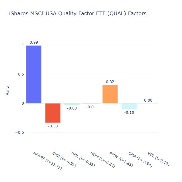
ETF Description: Selects large- and mid-cap stocks based on stable earnings growth and low debt-to-equity
Indeed, we see QUAL tilts toward profitability/quality (RMW = 0.32, t = 2.83) and towards larger companies (SMB = –0.33, t = –4.91). It seems to hold larger companies that are more likely to have stable earnings and robust balance sheets.
QGRO: American Century U.S. Quality Growth ETF
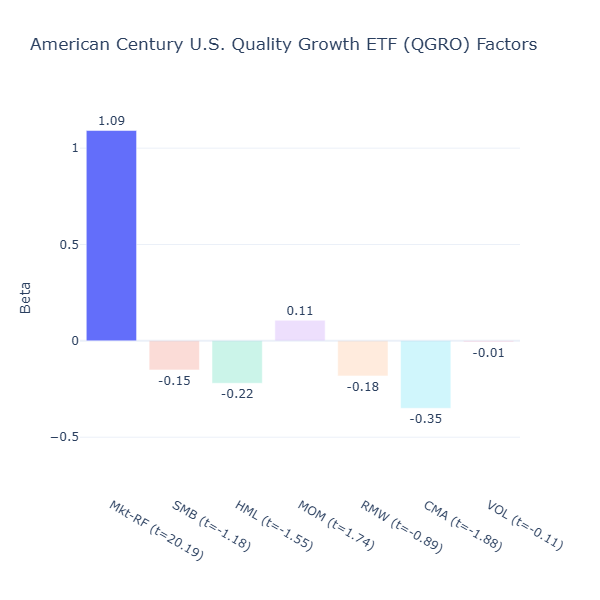
ETF Description: Tracks the American Century U.S. Quality Growth Index, selecting large- and mid-cap U.S. companies with strong quality, growth, and valuation fundamentals
Despite its name, QGRO does not seem to be meaningfully exposed to any of the factors to me, as of now.
Let’s look a bit more into its methodology by quoting its full description found here: “By focusing on larger companies with sound fundamentals and less volatility, QGRO attempts to mitigate some of the risk inherent in growth equities. The fund aims to have 35 percent to 65 percent of its portfolio in high-growth stocks, and 30 percent to 65 percent in so-called stable growth companies that exhibit attractive profitability and valuation. QGRO has a larger allocation to mid cap names than some single-factor quality and growth ETFs on the market, making it appealing for investors who want some diversification out of the large cap space.”
In practice, this can dilute any pure single‑factor exposure as these criteria can pull the portfolio in different directions. For example, the high‑growth allocation might overweight companies with weaker profitability but strong revenue growth, while the stable‑growth allocation might lean toward more profitable businesses When combined, these opposing tilts can effectively cancel each other out in a factor model, leaving no statistically significant exposure to any single factor.
Over time, its factor exposures may shift however, depending on which types of stocks pass its screen at each rebalance.
JQUA: JPMorgan U.S. Quality Factor ETF
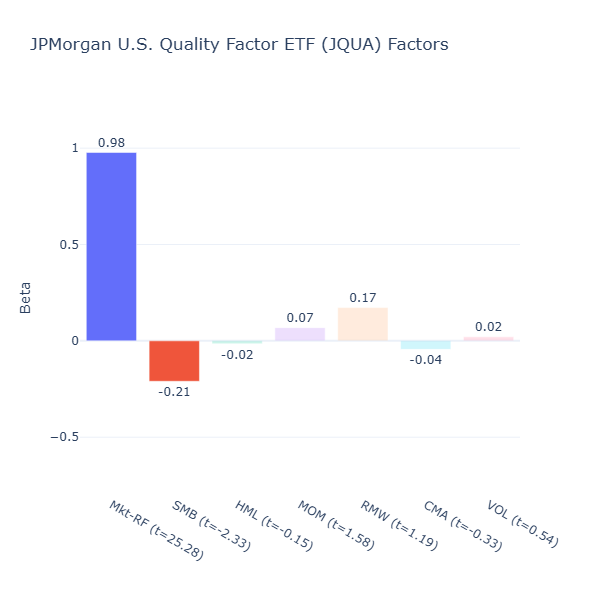
ETF Description: Selects U.S. stocks with high profitability, stable earnings growth, and low financial leverage to capture the quality premium
JQUA does not seem to be meaningfully exposed to any of the factors too, despite it being described as capturing U.S. stocks with high profitability. This is similar to QGRO in that the methodology may be too broad or diversified to produce a strong, measurable tilt in any one factor at the moment. While it screens for profitability, stable earnings growth, and low leverage, the combination of criteria (and possibly the current market environment) appears to have diluted the quality signal.
Comparing Among Quality‑Oriented ETFs
In this group, QUAL is the only ETF that currently delivers a clear, measurable tilt toward the quality factor in academic terms, profitability (RMW). It leans into large companies with stable earnings and strong balance sheets, making it a straightforward way to capture the quality premium.
By contrast, QGRO and JQUA do not show meaningful exposure to any factor at the moment. In both cases, their methodologies appear to be too broad or multi‑dimensional to produce a strong, consistent tilt.
It’s also worth noting that the definition of “quality” is not universal. In academic finance, the closest equivalent is the profitability factor (RMW), but asset managers may define quality more broadly — sometimes including stability, low leverage, or even valuation discipline. This flexibility means that two “quality” ETFs can look very different in their holdings and factor exposures.
Momentum ETFs
MTUM: iShares MSCI USA Momentum Factor ETF
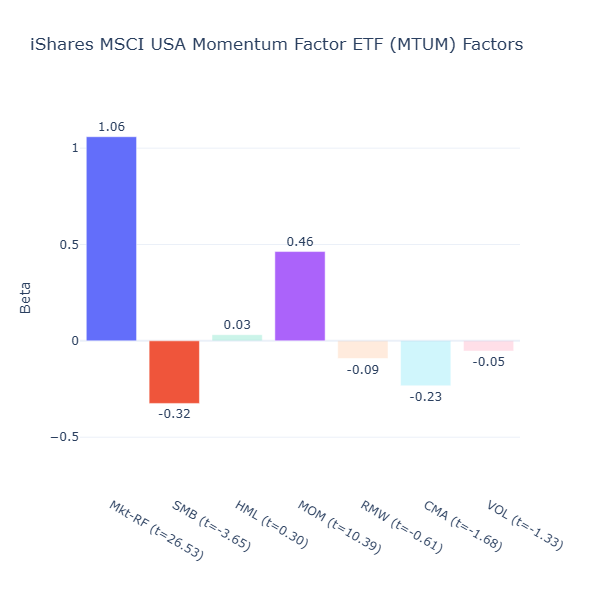
ETF Description: Holds large-cap U.S. stocks that exhibit positive price momentum
MTUM offers strong momentum (MOM = 0.46, t = 10.39) with a clear large cap tilt (SMB = –0.32, t = -3.65), which matches its description in a straightforward way.
VFMO: Vanguard U.S. Momentum Factor ETF
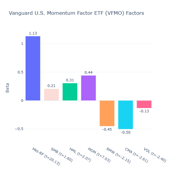
ETF Description: Tilts toward U.S. stocks exhibiting strong recent price momentum, selecting winners via a rules-based momentum screen
VFMO also has strong momentum (MOM = 0.44, t = 7.03) but adds other factor tilts: positive value (HML = 0.31, t = 2.07), strong negative profitability tilt (RMW = -0.45, t = -2.15) and strong aggressive investment tilt (CMA = -0.50, t = -2.61).
This is in stark contrast to MTUM, as VFMO also allows smaller, cheaper companies with negative profitability who are investing aggressively to make the cut. Some companies may even be in turnaround phases, not just mature, steady winners.
Comparing Among Momentum‑Oriented ETFs
As seen above, both funds provide strong momentum exposure, but the choice ultimately comes down to which type of momentum you want to capture. MTUM aligns more with larger, more-established momentum leaders. VFMO tilts toward smaller and cheaper names with strong momentum. Your preference depends on whether you value stability or are comfortable with a more aggressive momentum approach.
Low Volatility ETFs
USMV: iShares Edge MSCI Min Vol USA
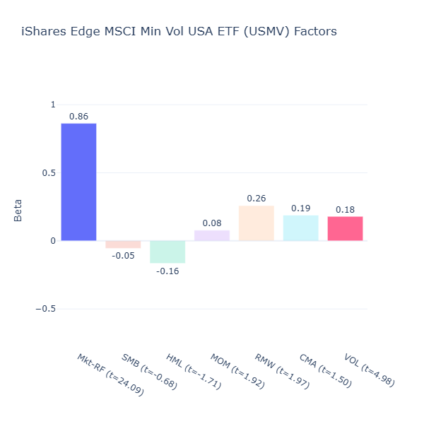
ETF Description: Tracks an index of U.S. stocks with the lowest realized volatility, aiming to smooth returns and reduce downside risk
USMV shows a positive low volatility tilt (VOL = 0.18, t = 4.98). We have not mentioned the market beta (Mkt-RF) before, but note that this ETF also the lowest beta for market returns that we have seen so far (Mkt-RF = 0.86).
Low volatility and beta for market returns are related, because a beta significantly below 1 means USMV tends to move less than the market, falling less in market downturns but also rising less in strong rallies, making it a steadier, smoother ride. This makes it a good defensive holding for investors who want to dampen portfolio swings.
SPLV: Invesco S&P 500 Low Volatility ETF
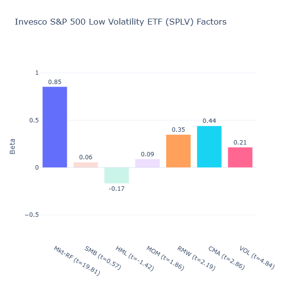
ETF Description: Selects the 100 least volatile stocks from the S&P 500
SPLV is also a low volatility ETF but it is built from the S&P 500 instead of the broader universe as in USMV. We see a similar low‑volatility tilt (VOL = 0.21, t = 4.84) and a lower market beta (Mkt-RF = 0.85) as USMV.
Interestingly, it has a positive profitability (CMA = 0.35, t = 2.19) and conservative investment tilt (CMA = 0.44, t = 2.86). The is because the S&P 500 is already a profitable, high‑quality large‑cap universe. When you take the 100 least volatile names from that pool, you end up with an even more concentrated set of stable, profitable companies which is often from defensive sectors like utilities, consumer staples, and healthcare.
Let’s do a quick verification on Google:
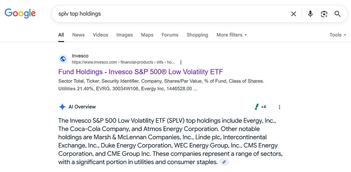
Defensive sectors tend to grow capacity slowly instead of investing aggressively because their demand is relatively stable and predictable.
Comparing Among Low‑Volatility‑Oriented ETFs
Both SPLV and USMV deliver on their promise of reducing volatility but they have some differences. USMV is a purer low‑volatility play with minimal exposure to other factors. Investors who are more comfortable with holding stable and profitable companies within the S&P 500 may prefer SPLV, but it likely also has less diversification than USMV, which is built from a broader universe.
Multi-Factor ETFs
LRGF: iShares US Equity Factor ETF
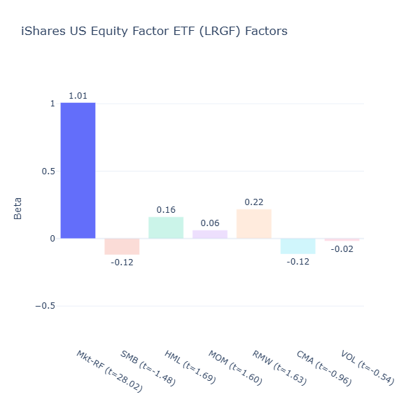
ETF Description: Selects large‑ and mid‑cap U.S. stocks to maximise exposure to momentum, quality, value, low volatility and size
LRGF spreads exposures fairly evenly, but factor tilts are generally mild, with no exposure reaching conventional 5% significance level (all t-values are < 2). Although this is consistent with its design to keep factor exposures balanced so no single one dominates, one might question whether such muted exposures truly deliver a distinct factor‑based return profile.
GSLC: Goldman Sachs ActiveBeta US Large Cap Equity ETF
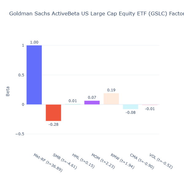
ETF Description: Targets value, momentum, quality and low volatility in large‑cap U.S. stocks
GSLC has a moderately negative size tilt (SMB = –0.28, t = –4.61) as it targets only large cap stocks. The rest of the factors are not significant. Like LRGF, GSLC aims for balanced exposure.
VFMF: Vanguard U.S. Multifactor ETF
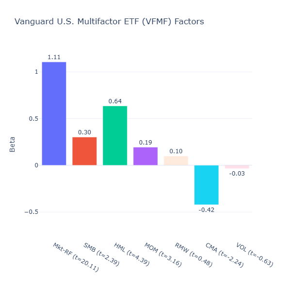
ETF Description: Tilts toward value, momentum, quality and low volatility across U.S. equities
VFMF is much more aggressive in its factor bets: strong positive value tilt (HML = 0.64, t = 4.39), positive size tilt (SMB = 0.30, t = 2.39), and positive momentum tilt (MOM = 0.19, t = 3.16). Interestingly, it also shows a strong negative investment tilt (CMA = –0.42, t = –2.24), indicating a preference for companies reinvesting aggressively. These small and aggressive companies with strong momentum can be volatile, so even though it tries to capture low volatility in its description, its low‑volatility exposure is negligible (VOL = -0.03, t = –0.63).
Comparing Across Multi‑Factor ETFs
It is not as straightforward to compare multi‑factor ETFs as it is for single or dual factor funds. Multi‑factor ETFs often follow more complex selection and weighting rules, which can produce a wide range of exposures depending on methodology and market conditions. While these rules may make sense from a portfolio construction standpoint, purely from a factor regression perspective one might question whether the muted exposures of LRGF and GSLC truly deliver a distinct factor‑based return profile.
LRGF and GSLC appear more suitable for investors seeking gentle diversification across several factors without straying far from core equity exposure, rather than those seeking strong factor convictions.
VFMF is more assertive, with statistically significant tilts toward value, size, and momentum, and a negative investment tilt that reflects its bias toward companies aggressively reinvesting. This makes it more suitable for investors who want stronger, clearly defined factor bets.
Ultimately, it is difficult for any multi‑factor ETF to deliver meaningful exposure to all factors at once without sacrificing some along the way. Of course, methodology choices can also prioritize certain factors over others, which is why multi‑factor funds can look so different despite sharing the same label.
Summary Heatmap of ETF Factor Betas
# boolean masks
mask_sig   = all_tstats.abs() >= 2
mask_insig = all_tstats.abs() <  2 # separate the statistically insignificant factors

plt.figure(figsize=(10, 8))
ax = sns.heatmap(
    all_betas,
    mask=mask_insig, # show only significant cells in rdgn color scheme
    annot=all_betas,
    fmt=".2f",
    cmap=rdgn,
    linewidths=0.5,
    cbar_kws={"label": "Beta"},
    annot_kws={"color":"black","alpha":1.0}
)

# overlay insignificant cells in light gray
sns.heatmap(
    all_betas,
    mask=mask_sig,         # show only insignificant cells here
    annot=all_betas,
    fmt=".2f",
    cmap=ListedColormap(["lightgray"]),  # gray background as betas are insignificant
    linewidths=0.5,
    cbar=False,
    annot_kws={"color":"gray","alpha":0.5}  # translucent gray text
)

# place xticks above and below
ax.xaxis.set_ticks_position('both')
ax.tick_params(axis='x', which='both', labeltop=True, labelbottom=True)

# draw horizontal dividers between categories
group_sizes = [2,3,5,3,2,2,4] # ok this is hardcoded to split the ETF into sectoions according to their categories
cum_sizes   = np.cumsum(group_sizes)

for y in cum_sizes[:-1]:
    ax.hlines(y, *ax.get_xlim(), color="black", linewidth=2)

plt.title("Heatmap of ETF Factor Betas")
plt.xlabel("Factors")
plt.ylabel("ETFs")
plt.tight_layout()
plt.show()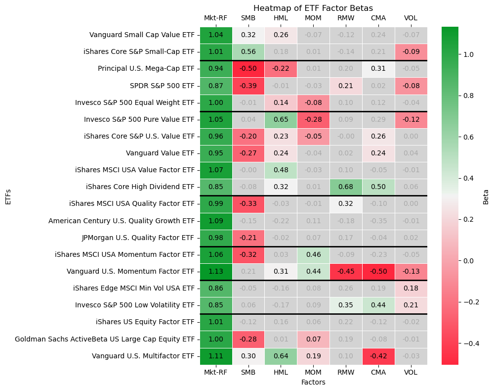
Let’s end off with a heatmap showing the factor betas for all ETFs we analyzed. I have added black horizontal lines to the heatmap to divide the ETFs into how we categorized them earlier: small‑cap, large‑cap/core market, value, quality, momentum, low volatility, and multi‑factor. Also:
Green cells represent a strong positive factor loading
Red cells represent a strong negative loading
Lighter colors mean the factor tilt is statistically insignificant (|t| < 2)
By scanning each column, you can see which ETFs share similar tilts, sometimes intentionally (e.g. all small‑cap ETFs showing significant SMB), and sometimes unintentionally (e.g. value ETFs occasionally picking up CMA also). This heatmap makes it much easier to spot overlaps and understand how different factor exposures combine across your portfolio if you decide to invest in them.
So are smart beta ETFs effective for factor investing?
The short answer is — yes, but only if you choose carefully, verify actual exposures, and understand the trade‑offs.
They Deliver Their Promises — But Rarely in Pure Form
Our regression analysis confirms that many Smart Beta ETFs do capture the factor tilts they advertise, value ETFs load positively on HML, momentum funds on MOM, and so on, especially the single or dual-factors ETF.
However, pure, isolated factor exposure is rare. Cross‑factor tilts are common, and some ETFs (especially those in the quality and multi‑factor categories) show muted or statistically insignificant loadings in the current market environment. Factor definitions themselves may also differ from ETF to ETF.
We have also seen that “broad market indexes” such as SPY, are not factor‑neutral; they have a large cap bias by construction, which can matter when blending them with other strategies. On the flip side, some funds, like VLUE, deliver exactly what they promise — a clean, straightforward value tilt that matches its name almost perfectly. So choose carefully.
The Long‑Only Effect and Market Exposure (Why Mkt-RF Has the Highest Beta)
We haven’t mentioned this, but it’s worth noting that long‑only Smart Beta ETFs can’t perfectly replicate academic factor portfolios. Academic models often go long the highest scoring stocks for a factor and short the lowest scoring ones (remember the “something minus something” names?). This design removes most of the returns from market exposure, isolating returns that come purely from the factor itself.
However, all of the above ETFs are long‑only, meaning they hold only the stocks they screen for and do not short the weakest names in a factor. As a result, market exposure is not removed and Mkt‑RF has the highest beta for all of them. This is not necessarily a bad thing, it means that while you tilt toward certain factors, you’re still getting a big part of the broad market risk and exposure in the ETFs, which historically has compounded upward over the long run.
This naturally dilutes betas and smooths out factor returns in real‑world implementation. This is why in the context of Smart Beta ETFs, I considered betas with 0.4 and above to be rather strong already, if you noticed. Of course, betas could have reached far higher values if they were allowed to short the stocks which rank the worst within each factor.
Verification Matters
Even though these ETFs largely follow rules based methodologies, factor tilts can drift over time due to rebalancing, sector rotations, or market cycles.
That’s why it’s essential to look beyond the marketing label of Smart Beta ETFs and verify the actual exposures as we’ve done here, if your aim is to use them for factor exposure. The heatmap and regression results give you a data‑driven view of what you’re really buying, so you can decide whether it aligns with your portfolio goals.
Final Takeaway
In my opinion, I would lean toward isolating a couple of high‑conviction factors and blend them with my core, since our analysis shows it’s hard for multi‑factor ETFs to give meaningful exposure to every factor without diluting the signal. A practical way to invest with Smart Beta ETFs is to start with a core market holding, something broad like the S&P 500 (SPY) or if you do not like its large cap bias, you can choose its equal‑weight version (RSP), to secure the broad market equity premium.
From there, layer in the factors you believe in most. If you think value will mean‑revert after years of underperformance, a clean value ETF like VLUE can tilt your portfolio toward cheaper stocks.
If you believe in trend‑following and want to ride market leaders, a momentum ETF like MTUM could be your choice. If you prefer defensive stability, a low‑volatility ETF like USMV might be suitable.
This way, you keep broad market participation while tilting toward styles that align with your market view and risk tolerance without chasing every factor at once.
👉 GET THE PYTHON NOTEBOOK for the full analysis in this post here.
Subscribe below now so you will be the first to be notified whenever I publish a new article!
Cheers,
Damian
Code Meets Capital