
Backtesting Fear and Greed Index As a Trading Signal
Do not be misled by the first set of results!

In a previous article, I did a deep dive into what the Fear & Greed index tells us about market returns with 14 years of data.
We also concluded that buying during extreme fear works best with a long holding period, while selling during extreme greed just to wait for the next “fear signal” to buy is unreliable and can make you miss entire bull market rallies.
As promised, I’ll now use the Fear & Greed Index as a trading signal in a backtest. But more importantly, we’ll uncover a dangerous trap: how blindly reading a heatmap of backtest results can be highly misleading if you don’t dig deeper.
👉 GET THE PYTHON NOTEBOOK for the full analysis in this post here.
Trading Backtest Setup
We’ll use VectorBT to run our backtests.
VectorBT is a fast and flexible Python library designed for backtesting and analyzing trading strategies with minimal code. It operates on signal-based logic, i.e. entries and exits are defined using simple boolean arrays, perfect for using indicators like the Fear & Greed Index. It also automatically calculates performance metrics such as returns, drawdowns, and more.
Here’s the setup:
import os
import numpy as np
import pandas as pd
import requests
import vectorbt as vbt # run "!pip install vectorbt" if you do not have it
import seaborn as sns
sns.set_theme() # to make the seaborn plots nicer
import matplotlib.pyplot as plt
# for coloring heatmap
from matplotlib.colors import LinearSegmentedColormap
from matplotlib.colors import TwoSlopeNorm
Get Fear and Greed Index Data
We combine historical data from both Part-Time Larry’s GitHub repo and CNN’s API, in the same manner described in the previous article.
# Old Fear and Greed index data from Part-Time Larry
url_old = 'https://raw.githubusercontent.com/hackingthemarkets/sentiment-fear-and-greed/master/datasets/fear-greed.csv'
df_old = pd.read_csv(url_old, parse_dates=['Date']).set_index('Date')
df_old = df_old.rename(columns={'Fear Greed': 'FG'})[['FG']]

# New Fear and Greed index data from CNN
start_date = (df_old.index.max() + pd.Timedelta(days=1)).strftime('%Y-%m-%d')
headers= {'User-Agent': 'Mozilla/5.0 (Windows NT 6.1; WOW64; rv:20.0) Gecko/20100101 Firefox/20.0'}
cnn_url = f"https://production.dataviz.cnn.io/index/fearandgreed/graphdata/{start_date}"
data = requests.get(cnn_url, headers = headers).json()['fear_and_greed_historical']['data']
df_new = pd.DataFrame(data)
df_new['Date'] = pd.to_datetime(df_new['x'], unit='ms')
df_new = df_new.set_index('Date').rename(columns={'y': 'FG'})[['FG']]

# Concatenate old and new data
df_fg = pd.concat([df_old, df_new]).sort_index()
df_fg.head()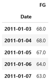
Obtain Historical Market Data (SPY) from Financial Modeling Prep API
Historical market data (SPY) can be obtained from the Financial Modeling Prep API for free. You need to sign up for an account here to get an API key.
Enter your API key in the next cell to store it in the environment variable “FMP_API_KEY”. We will use this for our requests below.
# uncomment and enter your FMP API Key inside
#os.environ['FMP_API_KEY'] = "YOUR_FMP_API_KEY"
from_date = df_fg.index.min().strftime('%Y-%m-%d') # only get data from the earliest date of fear and greed data available
symbol = 'SPY'
fmp_url = f"https://financialmodelingprep.com/api/v3/historical-price-full/{symbol}?from={from_date}&apikey={os.environ['FMP_API_KEY']}"
historical_spy = requests.get(fmp_url).json()['historical']
df_spy = pd.DataFrame(historical_spy).set_index('date')

# parse datetime and set as index
df_spy.index = pd.to_datetime(df_spy.index)
df_spy = df_spy['adjClose'].sort_index(ascending=True)
df_spy.head()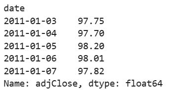
Align and Clean Data
Next, we will do some data cleaning by dropping duplicates for the Fear and Greed index data, as well as aligning its dates with the SPY prices dates to use in our backtest.
# drop any duplicates for Fear and Greed index data
df_fg = df_fg[~df_fg.index.duplicated(keep='last')]
# align Fear and Greed index dates with SPY dates
df_fg_aligned = df_fg['FG'].reindex(df_spy.index).ffill()
df_fg_aligned
We are now ready to run our backtests!
Run Backtests with the Following Scenarios
Here we’ll test different combinations of “buy when fear < X” and “sell when greed > Y” using VectorBT.
In particular:
enter when fear and greed index is lower than 10, 20, 30, 40 or 50
exit when fear and greed index is higher than 50, 60, 70, 80, or 90
entry_levels = np.arange(10, 51, 10)   # enter when fear and greed index is lower than 10, 20, 30, 40, 50
exit_levels  = np.arange(50, 91, 10)  # exit when fear and greed index is higher than 50, 60, 70, 80, 90
Now we will run our backtest by looping through each combination of entry and exit levels, passing them into vbt.Portfolio.from_signals().
VectorBT returns a whole list of tracking metrics for our backtests. For our purposes we will record a few metrics of interest into the records list, namely: ‘Total Return %’, ‘Max Drawdown %’, ‘Total Trades’ and ‘Benchmark %’.
def run_backtest(entry_levels, exit_levels, df_fg_aligned, df_spy):
    records = [] # list to append backtest result metrics
    for e in entry_levels:
        # enter and exit when fear greed  is above or below values defined above
        for x in exit_levels:
            entries = df_fg_aligned < e
            exits   = df_fg_aligned > x

            # run backtest using vector BT
            results = vbt.Portfolio.from_signals(
                close=df_spy, # close prices of SPY
                entries=entries,
                exits=exits,
                init_cash=100,
                freq='1D',
            )

            stats = results.stats() # stats for backtest
            # record metrics of interest
            records.append({
                'Entry': e,
                'Exit': x,
                'Return %': stats['Total Return [%]'],
                'Max Drawdown %': stats['Max Drawdown [%]'],
                'Total Trades': stats['Total Trades'],
                'Benchmark %': stats['Benchmark Return [%]'],

            })

    # create dataframe to store metrics of interest
    df_stats = pd.DataFrame(records)
    return df_stats

df_stats = run_backtest(entry_levels, exit_levels, df_fg_aligned, df_spy)
df_stats
Here are the results for each backtest:
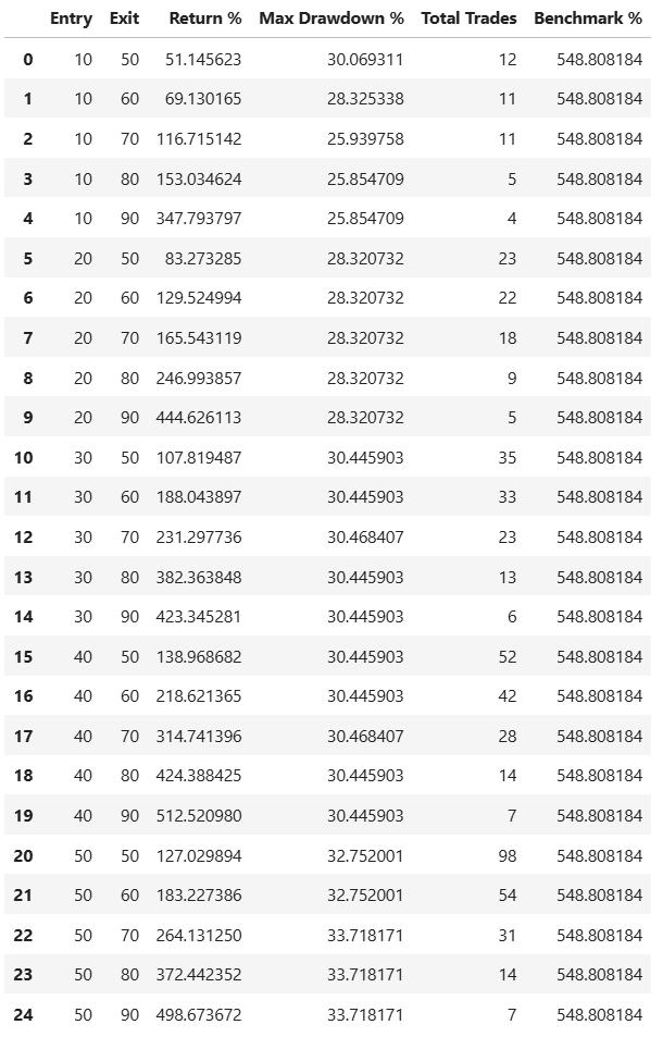
Firstly, the Benchmark % correspond to the returns for simply buying and holding SPY for the entire backtest period. It is 548.8%. We will keep that in mind.
The Max Drawdowns vary between 25% to 34%, without anything too drastic so we will ignore that for now.
The Returns vary widely between strategies, let’s visualize them on a heatmap.
Plot Results on Heatmap
We create a pivot table of our results and plot them on a heatmap.
# for coloring heatmap (darker shade of green for higher returns)
rdgn = sns.diverging_palette(h_neg=10, h_pos=130, s=99, l=55, sep=3, as_cmap=True)
divnorm = TwoSlopeNorm(vcenter=0)

# pivot data for heatmap (i.e. set Rows as Entry and Columns as Exit)
return_mat   = df_stats.pivot(index='Entry', columns='Exit', values='Return %' )
plt.figure(figsize=(5, 4))
sns.heatmap(
    return_mat,
    annot=True,
    fmt=".1f",
    cmap=rdgn,
    norm=divnorm,
    cbar_kws={'shrink': .8}
)
plt.title("Backtest Returns")
plt.ylabel('Entry When Fear Greed Below')
plt.xlabel('Exit When Fear Greed Above')
plt.tight_layout()
plt.show()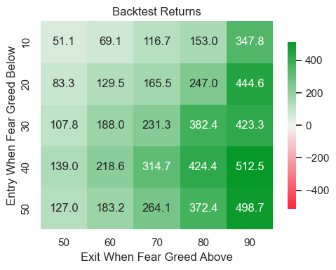
Be Careful — This Heatmap Can Mislead You!
Oops, from our heatmap, it seems like entering the market during extreme fear doesn’t perform that well.
In the first row,
buying when FGI < 10, even with the most patient exit atFGI > 90, the total return is only 347.8%, which is lower than strategies that buy at higher fear levels.This might appear to contradict what we found in the previous article — that buying during extreme fear leads to excellent long-term returns.
But the truth is:
This isn’t because buying at FGI < 10 is bad. It’s because you’re assuming you will often get the chance to buy at FGI < 10.
The Real Issue Is Waiting Too Long to Re-enter
In the backtest, after exiting at FGI > 90, we wait until the next FGI < 10 to buy again. But extreme fear (FGI < 10) happens very rarely — and sometimes not at all for years.
So by exiting during periods of Extreme Greed, you sit on the sidelines in cash, waiting for an Extreme Fear signal. Meanwhile, the market is climbing, and you’re missing out on years of gains.
So let’s test this:
What Happens If We Never Exit?
Include the Option to HOLD and NEVER EXIT
Let’s now re-run the backtest with an additional exit level: FGI > 100. The Fear & Greed Index never goes above 100, so this effectively means you never exit.
entry_levels = np.arange(10, 51, 10)
# What Has Changed?
# this time include exiting when Fear and Greed index is above 100, i.e. you HOLD and NEVER EXIT
exit_levels_new  = np.arange(50, 101, 10)

df_stats_new = run_backtest(entry_levels, exit_levels_new, df_fg_aligned, df_spy)# plot heatmap again

# pivot data for heatmap (i.e. set Rows as Entry and Columns as Exit)
return_mat   = df_stats_new.pivot(index='Entry', columns='Exit', values='Return %' )plt.figure(figsize=(5, 4))

sns.heatmap(
    return_mat,
    annot=True,
    fmt=".1f",
    cmap=rdgn,
    norm=divnorm,
    cbar_kws={'shrink': .8}
)

plt.title("Backtest Returns")
plt.ylabel('Entry When Fear Greed Below')
plt.xlabel('Exit When Fear Greed Above\n(Last Column is Hold and Never Exit)')
plt.tight_layout()
plt.show()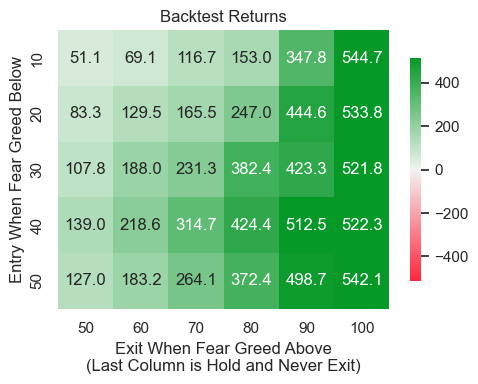
In the second heatmap, let’s look at the newly-added final column, Exit when FGI > 100 (i.e. buy and NEVER EXIT).
Suddenly, the
buying when FGI < 10strategy is the best performer, with a return of over 544.7% — the highest across the entire grid, in big contrast to the 347.8% returns in the second last column.As inferred from the last two columns, the difference in returns between
selling when FGI > 90to wait for re-entry during periods of fear, compared tonot selling at allis extreme.
Keep in mind that none of the “market-timing” strategies above beat the simple buy and hold benchmark of 548.8%, although buying where FGI < 10 came pretty close.
This tells us a few things:
Buying during Extreme Fear is still a great strategy. Even if you weren’t invested in the markets throughout this entire period, buying at
FGI < 10and then holding all the way came pretty close to the benchmark of being invested right from the start, despite a shorter holding period than the benchmark.Hence if I have spare cash lying around during periods of Extreme Fear, I will definitely consider putting them in the markets, if I am not already invested.
But do not treat Extreme Fear and Extreme Greed as trading signals. Exiting during extreme fear and waiting for rare fear signals to re-enter can severely hurt your returns.
Note: In the heatmap above, another high performing strategy seem to correspond to Entry when FGI < 50 , not because FGI < 50 is a magic threshold, but because these entries happened very near the start of the backtest period, with a longer holding period than other strategies and were allowed to compound over time.
Let’s now look at the Total Number of Trades.
Return vs Total Number of Trades in Strategy
Here we plot a scatterplot of Return % vs Number of Trades.
plt.figure(figsize=(6,4))
sns.scatterplot(data=df_stats_new, x='Total Trades', y='Return %')plt.title('Return % vs Number of Trades')
plt.xlabel('Number of Trades')
plt.ylabel('Return %')
plt.grid(True)
plt.tight_layout()
plt.show()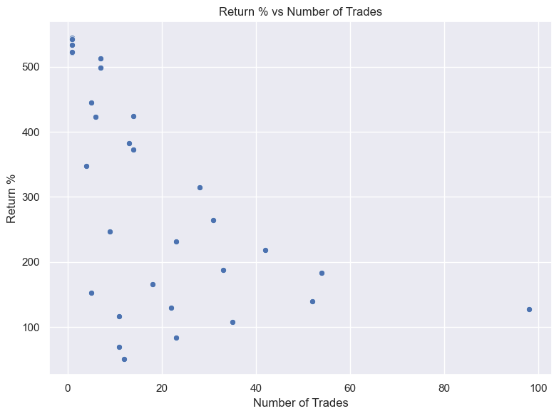
What we observe is a reinforcement of the idea that less trading = higher returns. The strategies that traded most frequently — reacting quickly to fear and greed shifts — often ended up with lower total returns. And we haven’t even factored in transaction costs.
In contrast, strategies that held for longer (e.g., with few exits or never exiting) are more likely to see compounding effects.
This finding supports the classic wisdom:
Time in Market Beats Timing the Market
While the Fear & Greed Index can help identify great entry points during periods of panic, it is often best paired with a strategy of patient holding — not active flipping based on sentiment alone.
Of course, this is not to say that all systematic trading strategies that trade most frequently are going to do badly, rather this is the case for trying to time the market using the Fear and Greed index.
Final Thoughts
Let’s go back to our initial conclusion in the previous article:
Buying during extreme fear works best with a long holding period, while selling during extreme greed just to wait for the next “fear signal” to buy is unreliable and can make you miss entire bull market rallies.
This conclusion holds true in our backtesting results.
However, if we had blindly looked for optimal entry and exit signals in our initial backtest criteria (enter when FGI < 10, 20, 30, 40 or 50 and exit when FGI > 50, 60, 70, 80, or 90), if we had stopped at the first heatmap, we would have falsely concluded that buying during extreme fear is worse than other signals.
Backtesting is powerful — but counterproductive if used without much thought.
Our initial heatmap made it look like buying during extreme fear (FGI < 10) was a bad strategy. But we eventually figured that we were waiting too long to re-enter. Extreme fear signals are rare. Sitting in cash while waiting for them means missing entire bull market runs.
When we modified the backtest to remove the exit condition, everything changed. Buying at FGI < 10 and simply holding nearly matched the benchmark return, even though it started later in the cycle. It wasn’t about perfect timing — it was about staying invested once you found a good entry.
Also, don’t be fooled by the strong results from “buy at FGI < 50” strategies and blindly conclude that they were the optimal entry signals. They performed well simply because they bought near the start of the backtest and held long enough to enjoy compounding returns.
Python Code
👉 GET THE PYTHON NOTEBOOK for the full analysis in this post here.